Real and complex signals
When doing the spectrum analysis, the signal is usually real-valued. However, when studying the baseband signal in wireless communications, the data is complex-valued. There is a significant difference in the processing of real and complex-valued signals for spectrum analysis.
You may notice the periodogram function in Matlab has an argument ‘freqrange’ that can be ‘onesided’, ‘twosided’, or ‘centered’. Similarly in matplotlib, the function pyplot.specgram has an argument ‘sides’ can be ‘onesided’ or ‘twosided’.
This is because, for real signals, the DFT results are mirrored (conjugated to be specific) at fs/2. In practice, only the spectrum from frequency 0 to fs/2 is shown. Note that, to make sure the energy of the displayed half spectrum is the same as the whole spectrum, the value of the half spectrum is doubled, except the DC.
As for complex-valued signals, the DFT results are useful from 0 to fs. The only thing we need to be cautious of is the frequency that is conventionally displayed from -fs/2 to fs/2. So when using periodogram in Matlab, it is recommended to set ‘centered’ instead of leaving default or ‘twosided’(0 to fs). Whereas matplotlib can take care of it by default.
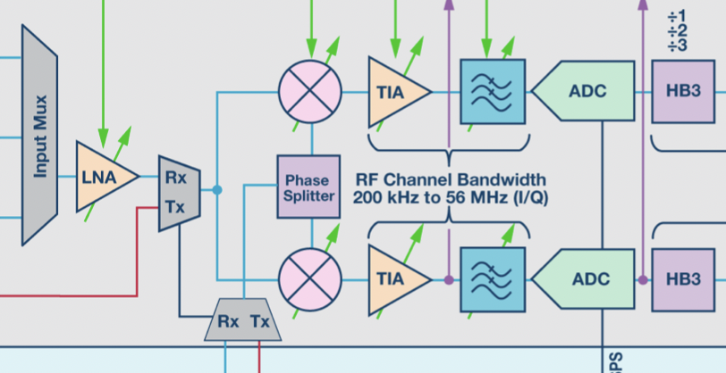
For example, if an SDR has a sampling rate of 56 MHz, the effective signal bandwidth is 56 MHz, not 28 MHz. Isn’t it breaking the Nyquist sampling theorem? If you take a look at a diagram of an SDR, you can find the incoming signal is separated into two channels and they are multiplied by a pair of orthogonal carriers, then, sampled by two ADCs to generate the IQ signal. We can not strictly consider each signal from one channel contributes half of the spectrum, so it is not violating the sampling theorem.

Parametric and nonparametric estimation
You may be told that the Periodogram or Welch methods for spectral estimation are nonparametric. In comparison, the Burg, Yule-Walker are parametric methods. What is the meaning of parametric anyway?
This term is from statistics, and there is a course called statistical signal processing, which I don’t excel at. So I am going to copy some text from this Matlab documentation page.
Parametric methods can yield higher resolutions than nonparametric methods in cases when the signal length is short. These methods use a different approach to spectral estimation; instead of trying to estimate the PSD directly from the data, they model the data as the output of a linear system driven by white noise and then attempt to estimate the parameters of that linear system.
If you get confused, just remember, the parametric methods believe the signal is generated from a model or follows the distribution of a model, and the spectrum is a function of the model parameters. The spectral estimation is then becoming a model parameter estimation problem.
For example, Burg and Yule-Walker methods assume an autoregressive (AR) model. The current date sample is a linear combination of a few previous samples and the noise. When it only depends on the last sample, it is equivalent to the Markov process.
If the model is chosen correctly, the parametric methods have better performance. This is due to the prior knowledge carried by the model and the reduced uncertainties brought by the noise. Just like the Bayes’ theorem, with the help of prior probability, we can yield a better posterior probability. This is assuming we have the right prior knowledge, otherwise, the likelihoods (nonparametric methods) are all we can rely on.
This reminds me of the concept of generative and discriminative models in machine learning. The generative classifiers try to find parameters for the prior distribution while the discriminative classifiers jump to the conditional probability directly.
That is all for now. Next time, I will bring some real Python code to compute the spectrum, spectrogram, and persistence spectrum.
Comments powered by Disqus.